A few months ago, I finished a machine learning project as a part of my mini project course last semester. I initially faced a lot of difficulties, since this was my first real machine learning project. You see, the whole process of machine learning involves a certain number of steps. Steps that you need to meticulously follow in a certain order so that the entire process is streamlined and efficient.

And that is exactly what I didn't do.

I'll write about everything that happened. It's gonna be long. And interesting. Maybe.

My aim was to find out, using machine learning, the eventual box office revenue of a movie. This would benefit production houses with multiple movies and advertising companies to know which movies to focus their budget on, to get the best return of investment. It would also help theatres to know which movies to showcase more if they knew beforehand if it was going to be succesful.

On a side note, as beginner in data science, this project was just not suited to me at all, since there were a lot of problems with the dataset. I wish I could look back and say I learned a lot, but the truth is I don't think I will ever need the information I learnt in the near future, and when I will, I would've forgot what I learnt.

The first mistake I did. I never learned from a concrete source. All I did was learn from multiple sources like a maniacal autodidact. Now the problem here was that since I was learning from multiple sources, I did not know the difference between inference and prediction. In short, prediction doesn't need Gaussian assumptions of algorithms to be fulfilled. But inference does. Whenever I googled 'linear regression', every website stressed the importance of fulfulling assumptions but no one said it was meant for inference.

Inference here means knowing what features affect prediction results and how exactly they affect them. For example, to do this accurately with linear regression, these assumptions need to be fulfilled:

• The statistical distribution of your dependent variable (revenue in this case) has to be normally distributed. Now this isn't compulsory but many sources stressed it.
• Your residuals should have constant variance, i.e. they should be homoscedastic.
• There should be no multicollinearity between your features.
• The independent variables and dependent variable should have a linear relationship between them.

I chased after these assumptions like Tom chases Jerry. But to no avail. All I cared about was prediction. But I carried out inference. I used correlation heatmaps and the Variance Inflation Factor to mitigate multicollinearity. I conducted Breusch Pagan tests and white tests to test for heteroscedasticity. I looked for hours at the residual scatter plot trying to achieve the holy grail of homoscedasticity but I just couldn't manage to achieve it. I tried a variety of solutions:

• Using weighted regression
• Applying variance stabilizing transformations
• Log-transforming the dependent variable
• Box-Cox transformations

BUT. NONE. OF. THEM. WORKED. :(

As I was also learning at the same time I was doing the project, I wasted a LOT of time. Time I could never get back. Sigh. But on the bright side, I finally did find out what to do. I will forever be grateful to that one redditor who pointed me in the right direction. I quickly got back on track after that. Thank you, stranger.

I used two datasets from Kaggle. Dataset1 had 45,000 samples and Dataset2 had 5000. I did an inner join on them using the IMDb ID column to combine both datsets. I did this in order to hopefully get a better prediction due to more number of features. Although this isn't a good idea in some cases. If you have a crap-ton of features, the algorithm needs more computer resources for execution, and there is a possibility of multicollinearity affecting prediction. This is the reason why dimensionality reduction techniques exist. Too much of something is not good.

Except money of course.

Since two datasets were merged, columns like revenue were repeated- one from each dataset. However there were some discrepancies. Turns out the difference between these columns were 43%.

(abs(movies['revenue'] - movies['gross']) / (movies['revenue'] + movies['gross']) * 100).mean()

Why was that? After manually googling a randomly sampled movie and checking out its revenue, I found out that one dataset contained global revenue and another contained revenue for the U.S. only. Since I want the scope of the project to be simple, I decided to use the column with U.S. revenue and discard the other.

movies = movies[movies['production_countries'].apply(lambda x: True if 'United States of America' in x else False)]
movies = movies[movies['spoken_languages'].apply(lambda x: True if 'English' in x else False)]

Next, genre. There were yet again two more the of the same columns. I discarded the column with a lower SPRF (self-proclaimed-relevance-factor), which I define as the average number of genres listed per movie. How this helps in my case I do not yet know. Dataset1 had the genres in an unusual format on which I had to use literal_eval to extract information and extracting the genre from Dataset2 was easy enough, all I used was a split() function. Looking at their individial SPRFs, Dataset2 had more information so I chose to go alone with that and discard the genre column from Dataset1.

print(movies['genres_x'].fillna('[]').apply(literal_eval).apply(lambda x: len([i['name'] for i in x]) if isinstance(x, list) else []).mean())
print(movies['genres_y'].apply(lambda x: len(x.split("|"))).mean())

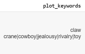
This next step contradicts my previous step. I will filter out and use only one genre. While knowing all the genres of a movie might help in building something like a movie recommender system, I do not see the point in using each listed genre of a movie for this project. There was also a feature which listed plot keywords, which would be a massive boon in recommender systems. But then again, that's not the goal here. (I also don't know how to build one). Guess which movie this is referring to:

I then converted the release dates which were objects to a datetime format for convenience.

months = ['Placeholder', 'Jan', 'Feb', 'Mar', 'Apr', 'May', 'Jun', 'Jul', 'Aug', 'Sep', 'Oct', 'Nov', 'Dec']
movies['release_date'] = movies['release_date'].apply(lambda x: datetime.strptime(x, '%Y-%m-%d'))
movies['release_month'] = movies['release_date'].apply(lambda x: months[x.month])
movies['release_year'] = movies['release_date'].apply(lambda x: x.year)

Converted other columns to a list format which made things simpler:

movies['production_companies'] = movies['production_companies'].fillna('[]').apply(literal_eval).apply(lambda x: [i['name'] for i in x] if isinstance(x, list) else [])
movies['production_countries'] = movies['production_countries'].fillna('[]').apply(literal_eval).apply(lambda x: [i['name'] for i in x] if isinstance(x, list) else [])
movies['spoken_languages'] = movies['spoken_languages'].fillna('[]').apply(literal_eval).apply(lambda x: [i['name'] for i in x] if isinstance(x, list) else [])

I then proceeded to drop rows with NA values and then the columns which wouldn't be needed. These wouldn't assist us in prediction for now. Most of these were either repeated columns due to merging of datasets or they were in string formats which I currently do not know how to incorporate as variables. Probably something to do with Natural Language Processing though.

columns_to_drop = ['revenue', 'movie_imdb_link', 'genres_x', 'genres_y', 'homepage', 'id', 'imdb_id', 'overview',
                   'poster_path', 'status', 'tagline', 'movie_title', 'original_language', 'original_title', 'video',
                  'budget_x', 'language', 'country', 'adult', 'plot_keywords', 'aspect_ratio', 'runtime', 'title_year']

movies = movies.drop(columns_to_drop, axis = 1).rename(columns = {'budget_y' : 'budget', 'gross' : 'revenue'})

First step was the usual summary statistics. Nothing out of the ordinary. In total, I had 3943 movies to work with, and the summary looked normal.

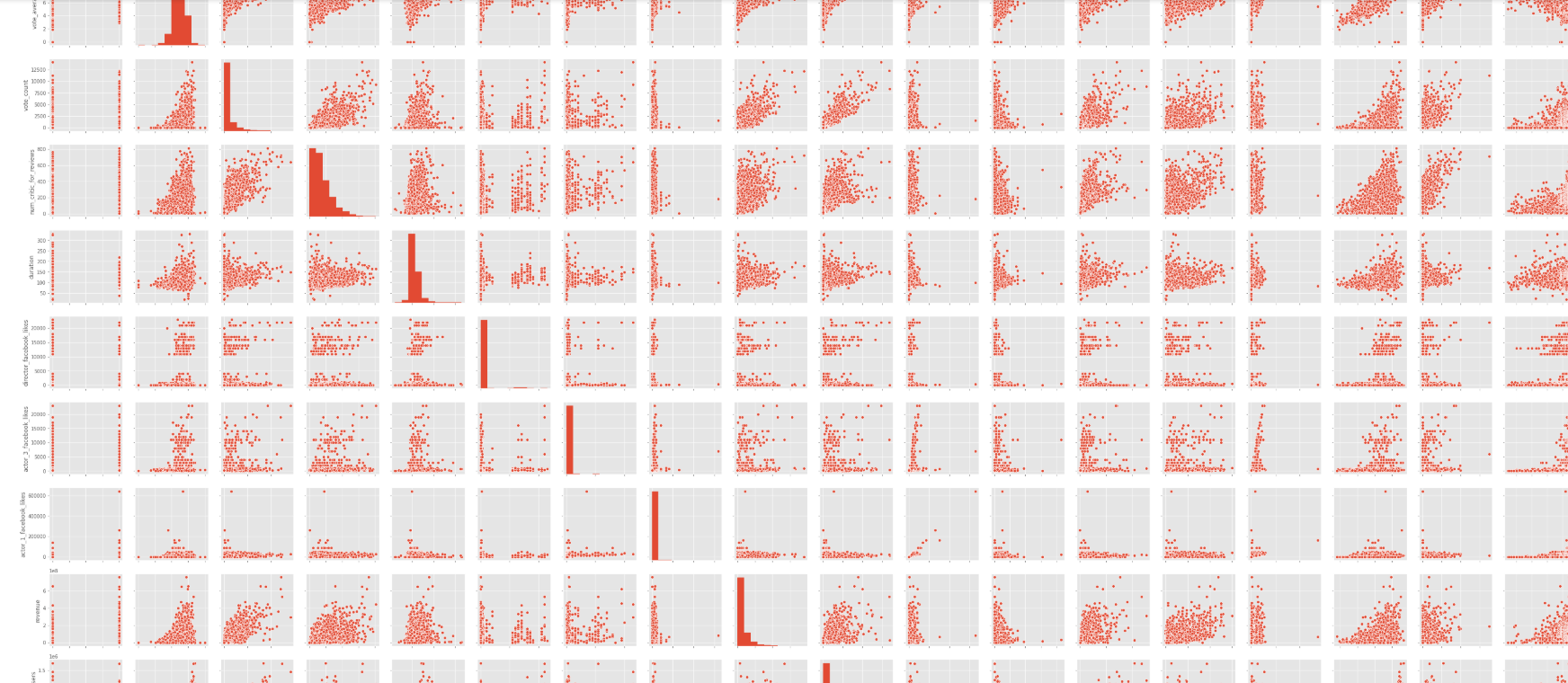
I took a pairplot and I can infer nothing from this except the fact that it looks kinda cool:

Looking at the distribution of the dependent variable, revenue, we can see that it exhibits a Pareto distribution. Right now it's beyond my scope to understand what a Pareto distribution actually is. Though as you can see, the distribution isn't normal. If you take log of the values, you will ensure normality but this made a lot more problems down the line that I wasn't equipped to handle. And as mentioned before, since this is just prediction, normality won't matter.

Next, looking at the barplot of the number of movies released each year, we can see that the bulk of the graph is towards the right. I'll take 1995 as the cutoff year, i.e. only taking movies released after 1995 into account.Why?

• We don't have a lot of movies released before around the 1995 mark.
• The budgets/revenue are not adjusted for inflation over time.
• Movies of the previous century tend to be different than the movies of the 2000s in a lot of ways. For instance, the budget allocated for movies after 2000 would be much more than ones before 2000. Again, inflation probably plays a role here but for simplicity I will not be working with the old movies.

Looking at the overall budgets each year, I could've taken 1990 but it had a few empty values for some months- which I found using a heatmap, so I chose 1995.

pd.DataFrame(movies.groupby('release_year').sum()['budget']).tail(25)

Looking at a heatmap of the revenue over different months of different years, we can see that most revenue is made in the months May, June, July, November, and December.

According to the internet:

Woo! Exciting! Never tried this before, however I made three very basic features. The model accuracy did improve, however it was by a very small amount. More on that later. The features I engineered were:

• action_or_adventure: The revenue across different genres were studied upon. Upon visual analysis, it was found that Action and Adventure movies on average earned more revenue when compared to other genres. Thus, a new column was created, which contains a 1 if the genre of the movie is either action/adventure, else contains a 0. I'm not statisically sound yet, but I do know that the error bars here represent the level of uncertainty for that particular genre. Taking that into account, we're left with action and adventure genres.

movies_numerical['action_or_adventure'] = movies['genre'].apply(lambda x: 1 if x == 'Action' or x == 'Adventure' else 0)

• top_director: The top 10 directors sorted in descending order by average revenue per movie were used to create a new column, called top_director, which contains a 1 if the director of that particular movie is a top director, else contains a 0.

top_10_directors = list(movies.groupby('director_name').sum().sort_values(by = 'revenue', ascending = False).head(10).reset_index()['director_name'])
top_10_directors_revenue = list(movies.groupby('director_name').sum().sort_values(by = 'revenue', ascending = False).head(10).reset_index()['revenue'])
directors_and_revenue_dict = dict(zip(top_10_directors, top_10_directors_revenue))
movies_numerical['top_director'] = movies['director_name'].apply(lambda x: 1 if x in top_10_directors else 0)

The top 10 directors are:

Steven Spielberg! No surprise there.

According to the interwebs:

First thing I did for feature selection was to conduct backward elimination. Backward elimination is an iterative process starting with all variables and in each iteration, deleting the variable whose loss gives the most statistically insignificant deterioration of the model fit, and repeating this process until no further variables can be deleted without a statistically significant loss of fit. Here, the probability value (p-value) was used. In simple terms, if the p-value of a certain feature is 0.05, then it means that there is a 5% chance that the results obtained were due to pure chance rather than due to the statistical features of the data. Overall, three features were removed after doing backward elimination 3 times. These feature were facenumber_in_poster, num_critic_for_reviews, and release_year. The backward elimination itself was done using statsmodels OLS, which required that the constant of the linear regression equation be added manually.

X = movies_numerical.loc[:, movies_numerical.columns != 'revenue']
Y = movies_numerical['revenue']
X_train, X_test, Y_train, Y_test = train_test_split(X, Y, test_size = 20)
model = LinearRegression(fit_intercept = True)
model.fit(X_train, Y_train)#, sample_weight = self.sample_weight)

movies_with_intercept = movies_numerical.copy()
movies_with_intercept['intercept'] = model.intercept_
X = movies_with_intercept .loc[:, movies_with_intercept .columns != 'revenue']
Y = movies_with_intercept ['revenue']
insignificant_cols = ['facenumber_in_poster', 'num_critic_for_reviews', 'release_year']
X = X.drop(insignificant_cols, axis = 1)
regressor_OLS = sm.OLS(endog = Y, exog = X, hasconst = True).fit()
regressor_OLS.summary()

Multicollinearity is when a feature may be correlated with another feature. For inference, this needs to be removed. Why? If two variables contribute approximately the same to the dependent variable's outcome, it's useless to use both since we cannot measure individual contribution and importance of a single variable. The heatmap below shows that multicollinearity indeed exists but I will not be removing them. As I've mentioned before, I don't care about it when it comes to prediction.

Finally! The part everyone's been waiting for. Nothing too complicated, just split the datasets into testing and training sets and ran them through a plethora of regression algorithms:

Linear Regression: Multiple linear regression is a technique that uses multiple explanatory variables to predict the outcome of a single response variable through modeling the linear relationship between them. It is represented by the equation below:

Support Vector Regression: A Support Vector Machine is a classifier that aims to find the optimal hyper-plane (the separation line between the data classes with the error threshold value epsilon) by maximizing the margin (the boundary between classes and that which has the most distance between the nearest data point and the hyper-plane). In this project, a linear kernel was used.

Decision Tree Regression: A decision tree is a supervised classification model that predicts by learning de-cision rules from features. It breaks down data into smaller subsets by making a decision based on asking a series of questions (the answers are either True or False), until the model gets confident enough to make a prediction. The end result is a tree, where the leaf nodes are the decisions. The questions asked at each node to determine the split are different for classi-fication and regression. For regression, the algorithm will first pick a value, and split the data into two subsets. For each subset, it calculates the MSE (mean squared error). The tree chooses the value with the smallest MSE value. After training, the algorithm runs it through the tree until it reaches a leaf node. The final prediction is the average of the value of the dependent variable in that leaf node. The usage of a single decision tree gave the worst results. While decision trees are supposed to be robust against collinearity, they did not perform better than linear regression.

Random Forest Regression: Random forest is an ensemble method, which means that it combines predictions from multiple machine learning algorithms, in this case, decision trees. The problem with decision trees is that they are very sensitive to training data and carry a big risk of overfitting. They also tend to find the local optima, as once they have made a decision, they cannot go back. This was evident by the fact that the R² value and correlation varied in each iteration of running the algorithm. Random forest contains multiple decision trees running in parallel, and in the end, averages the results of multiple predictions. Random forests with 100 trees were found to have the best results among all algorithms used in this project.

Ridge Regression: Ridge regression L2 uses regularization, which is a method used to avoid over-fitting by penalizing high-valued regression coefficients through shrinkage, where extreme values are shrunk towards a certain value. Particularly, In L2 regularization, the coefficients are penalized towards the square of the magnitude of the coefficients. Ridge regression is a technique used to mitigate multicollinearity in linear re-gression. While the fulfillment of the multi-collinearity assumption is not necessary for prediction and is only necessary for inference, using Ridge Regression decreased performance. The cause of this was not clear.

Lasso Regression: Similar to ridge regression, lasso regression shrinks all coefficients towards a value, in this case, the absolute value of the magnitude of coefficients. This is called L1 regularization, and can sometimes lead to elimination of some coeffi-cients. Lasso regression had similar performance to Ridge regression.

The metrics used to measure the efficacy of these algorithms were:

• Mean Absolute Error
• Mean Squared Error
• Root Mean Squared Error
• R² (coefficient of determination)

Not immediately clear which algorithm performs better. By visually representing them, we can see it better. Since correlation and R² are on different scales, I will seperate them from the rest of the metrics.

Looking at the results above, we can see that Random Forest had the best performance out of all the algorithms. The next best algorithm was linear regression, due to it's low error scores.

While looking at different blogs on the internet, I came upon something called feature_importances, which basically means the features most responsible for determining the revenue of a movie. This was done using Random Forest Regressor. In each individual tree in the forest, the decision is made based on the MSE (Mean Squared Error). When training individual trees, the degree of how each feature decreases the MSE can be averaged. The features are then ranked accordingly in ascending order.

According to this, the number of votes garnered online and the budget allocated for a movie were the most important in determining the overall revenue of a movie.

Phew! My first ever full fledged machine learning project. Went kinda good, except for the statistical roadblocks, and the lack of a path. Guess this is what machine learning projects are all about- you need to have statistical knowledge, and a concrete sequential way of doing things. I have a lot of studying to do. I'm almost sure that somewhere in my code I've messed up (statistically, that is) which causes my results to be inaccurate. Well. That's something to worry about in the future.

From the stars,
FR.