Hey. Been a while. Wanted to dip my hands into a new grid-based project since the one I built with p5.js (A Conway's Game of Life visualizer), was sub-optimal in terms of performance. You can check it out here. . It suffers when the resolution is too high. I suspect it's due to the bad way the screen updates (every single pixel is re-rendered, instead of re-rendering only the ones that need to be updated). I tried looking at past-me's code and I gagged. So I decided to make an entirely new project entirely.
Building a pathfinding visualizer has been on my list for a long time, ever since I came to know of Clement Mihailescu's Pathfinding Visualizer . I've built a sorting visualizer that works pretty well, so the only thing left really was a pathfinding visualizer. I was scared of graph algorithms for a long while, but it's LeetCode season, and seeing how easy DFS and BFS were to understand, I decided to finally delve into this. And I can say that it was not at all as complicated as I expected it to be. A year ago I would not have been able to. Never undermine yourself. Times change. And so do people. (Is this becoming a motivational blog?)
What's the stack, you ask? Pygame. That's it. Literally, nothing else. If this was web development then I probably would have used p5.js, but Python is near and dear to my heart and it was time I finally built something using PyGame. Only disadvantage is the barrier to entry for people who want to play with this project themselves (which, is pretty easy enough. Clone the repo , run the code.). Nevertheless, for the laymen out there, or in general people who can't be bothered with trying to get the code running themselves, I will do my best in explaining how this project was built from the ground-up and all the design decisions that went into it.
Drawing an empty board
The way the project is set up is we have the entire board, represented by the class Lattice, which is made up of an nxn grid, where each unit is a Node. Each Node contains information about it's row and column number. PyGame takes this information, and also information about the node side length (which is a static value), and draws rectangles, populating the entire Lattice with tiny little squares. I went ahead with the decision of not having any visible border, because in my opinion, it just looks ugly. The colour of the node is also dependent upon it's state. On an empty board, all nodes have the state NodeState.VACANT, which is represented by an Enum class. I've put all this into a draw() function, which is used in situations when you need to update the entire state of the lattice (i.e. all nodes) in one single update. Here's the bulk of the draw function, but remember, a lot of it is abstracted. If you're interested you can just check out the code yourself.
def get_rect_from_node(self, node: Node) -> pg.rect.Rect:
    x, y = self.get_node_coords(node)
    render_number = self.previously_rendered_nodes.get(node, None)
    colour = node.get_colour(render_number)
    rect = pg.draw.rect(
        self.pg_screen,
        colour,
        pg.Rect(x, y, self.info.node_size, self.info.node_size),
    )
    return rect

def draw(self) -> None:
    new_rects = []
    for r in range(self.nrows):
        for c in range(self.ncols):
            node = self.get_node(r, c)
            new_rect = self.get_rect_from_node(node)
            new_rects.append(new_rect)
    pg.display.update(new_rects)  # type: ignore
We'll get to what render_number means later on. For now, it's not important. If you noticed, I use pygame.display.update() instead of pygame.display.flip() . This is much more efficient, since flip() re-draws the entire screen, while update() only updates the areas of the screen which need to be updated. How does it know this? For this project atleast, it's through the list of Rect objects we pass as a parameter to update().
The Node class
This is the fundamental unit of the board. Think: atom. Yeah, revolutionary. The entire grid is just a bunch of Nodes arranged in order. Each node has some important information, which you will see below. I have omitted a bunch of getters and setters, because they're not necessary for this post.
class Node:
    def __init__(self, pos: Pos, state: NodeState = NodeState.VACANT) -> None:
        self.state = state # Can be one of each: VACANT, WALL, ORIGIN, GOAL, VISITED, PATH
        self.pos = pos # A namedtuple: Pos(r, c), which contains a node's row and column number
        self.heuristic = None # The euclidean distance between a node and the origin node, used in A star search
        self.predecessor = None # The node that came before this node in a pathfinding traversal
        self.already_rendered = False # Used in colour gradient rendering. More on this later.

    def get_colour(self, render_number: int) -> str:
        if render_number is None:
            return node_colours[self.state][0]
        return node_colours[self.state][render_number - 1]

    def reset(self) -> None:
        self.state = NodeState.VACANT
        self.predecessor = None
The function get_colour() is important, because it is responsible for setting the colour of the node, depending on two things: it's state, and which loop it was rendered in. To make the grid look better during a pathfinding visualization, I have set it up so that with each update i.e. everytime a node is visited, the colour of the nodes that were previously rendered slowly transition into a base colour. This would give us an idea of how the visualization is progressing.
Only two states have this colour transition property: PATH, and VISITED. For each of these nodes, I have specified a range of colours. Using the colour module python, I take these range of colours, and generate more colours. For a smooth transition, the number of colours has to be high. I have found that 1000 colours is a good number, considering the trade-off between good visuals, and memory needed (the more colours there are, the more updates are made to the screen. And the more updates there are, the slower the visualization occurs, due to the fact tha PyGame only uses the CPU and not the GPU).
Here are the specified colours for each of the states:
node_colour_ranges = {
    NodeState.WALL: ['#000500'],
    NodeState.VACANT: ['#FAF0CA'],
    NodeState.ORIGIN: ['green'],
    NodeState.GOAL: ['red'],
    NodeState.VISITED: [
        '16DB65',
        '058C42',
        '04471C',
    ],
    NodeState.PATH: ['#ffd100', '#ffee32'],
}
If a state has only one colour, it means it does not change as more renders happen. It does not make sense to change colours for wall nodes or the origin/goal node, because these stay in the same place and offer us no information about how the pathfinding is progressing.
These colours are taken, and expanded into a much bigger list, where the start and end colours are the same, but the colours in between are generated to gradually transition. The code for this is a bit convoluted because I account for a variety of edge cases, and I wanted to make changing colour schemes easy. All I have to do to specify new gradient colours is to update the node_colour_ranges object above, and the chunk of code below does all of the work for me.
node_colours = {}
for node_state, colour_range_colours in node_colour_ranges.items():
    num_colours_in_colour_range = len(colour_range_colours)
    if num_colours_in_colour_range > 1:
        colours = []
        for i in range(num_colours_in_colour_range):
            if i + 1 < num_colours_in_colour_range:
                start_colour = colour_range_colours[i]
                start_colour = f'{"#" if "#" not in start_colour else ""}{start_colour}'  # Handles case if # is not present in specified colour range hex value
                end_colour = colour_range_colours[i + 1]
                end_colour = f'{"#" if "#" not in end_colour else ""}{end_colour}'
                colours.extend(
                    map(
                        lambda color: color.hex_l,
                        Color(start_colour).range_to(
                            Color(end_colour),
                            NUM_COLOURS_IN_TRANSITION
                            // (num_colours_in_colour_range - 1)
                            if num_colours_in_colour_range > 2
                            else NUM_COLOURS_IN_TRANSITION,
                        ),
                    )
                )
        # The 3 lines below are only needed because if there are more than 2 colours in a given NodeState's colour transition,
        # the above code that adds the colour gradient between two colours doesn't exactly sum up to NUM_COLOURS_IN_TRANSITION
        # at the end. This means the last few colours in a given transition will be the same, but it is pretty much
        # unnoticeable if the value of NUM_COLOURS_IN_TRANSITION is high
        num_colours_left = NUM_COLOURS_IN_TRANSITION - len(colours)
        fillers = [colours[len(colours) - 1] for _ in range(num_colours_left)]
        colours.extend(fillers)
        node_colours[node_state] = colours
    else:
        node_colours[node_state] = colour_range_colours
This node_colours object is what is used in the get_colour() function of the Node. Depending on the render number (after which a certain node was rendered), this new list node_colours is indexed. Since we chose 1000 colours to be present in this list, a node's colour would change each time a pygame.display.update() is called, for upto a 1000 times. After this, it is no longer updated. This does mean that as the visualization progresses, more nodes are rendered, leading to a slight performance decrease as time goes on. But for the purposes of this experiment, and in general, unless your node size is too small or your grid size is too big, this won't be much of a problem. Performance enhancements beyond pygame.display.update() are inconceivable to me. The only improvements that can be made is in how the pathfinding algorithms are themselves written, which we will get to in a bit.
The Lattice Class
Arguably, I could have done a better job in modularizing this class, specifically, I could have moved the algorithm functions to a separate module or class, but I think the size of the class is just right to not warrant an improvement anytime soon. At the time of writing this, it spans 700 lines, which isn't too bad. If I add more algorithms after this, I will write them out into a separate class/module. As of writing this (Dec 3rd, 2022), all the algorithms it has are BFS, DFS, Dijkstra, A*, Game of Life, and Maze Generation.
The Lattice is initialized with Nodes, the number of which are specified by the value in the static variables in main.py, SCREEN_SIDE_LEN. The following is the __init__ function for the lattice.
class Lattice:
    def __init__(self, pg_screen: pg.surface.Surface, lattice_info) -> None:
        self.values = []
        self.info = lattice_info
        self.draw_mode = DrawMode.SET_WALL
        self.ncols = lattice_info.screen_dim.w // lattice_info.node_size
        self.nrows = lattice_info.screen_dim.h // lattice_info.node_size
        self.origin = None
        self.goal = None
        self.pg_screen = pg_screen
        self.previously_rendered_nodes = (
            {}
        )  # Contains nodes which have been rendered since beginning of the animation. Used to enable gradient animation on nodes as visualization progresses

        for r in range(self.nrows):
            row = []
            for c in range(self.ncols):
                row.append(Node(Pos(r, c)))
            self.values.append(row)
lattice_info is a namedtuple that contains the following information: screen_dimensions, and node size. previously_rendered_nodes is a dictionary where the key is a Node object and it's value is an integer. It contains nodes which exist in the renders from 0 (a node's inception), till the number NUM_COLOURS_IN_TRANSITION. Once a node has been through enough renders (such that it's colour returns to the end colour in our custom specified range), it is removed from this dictionary.
Drawing Walls
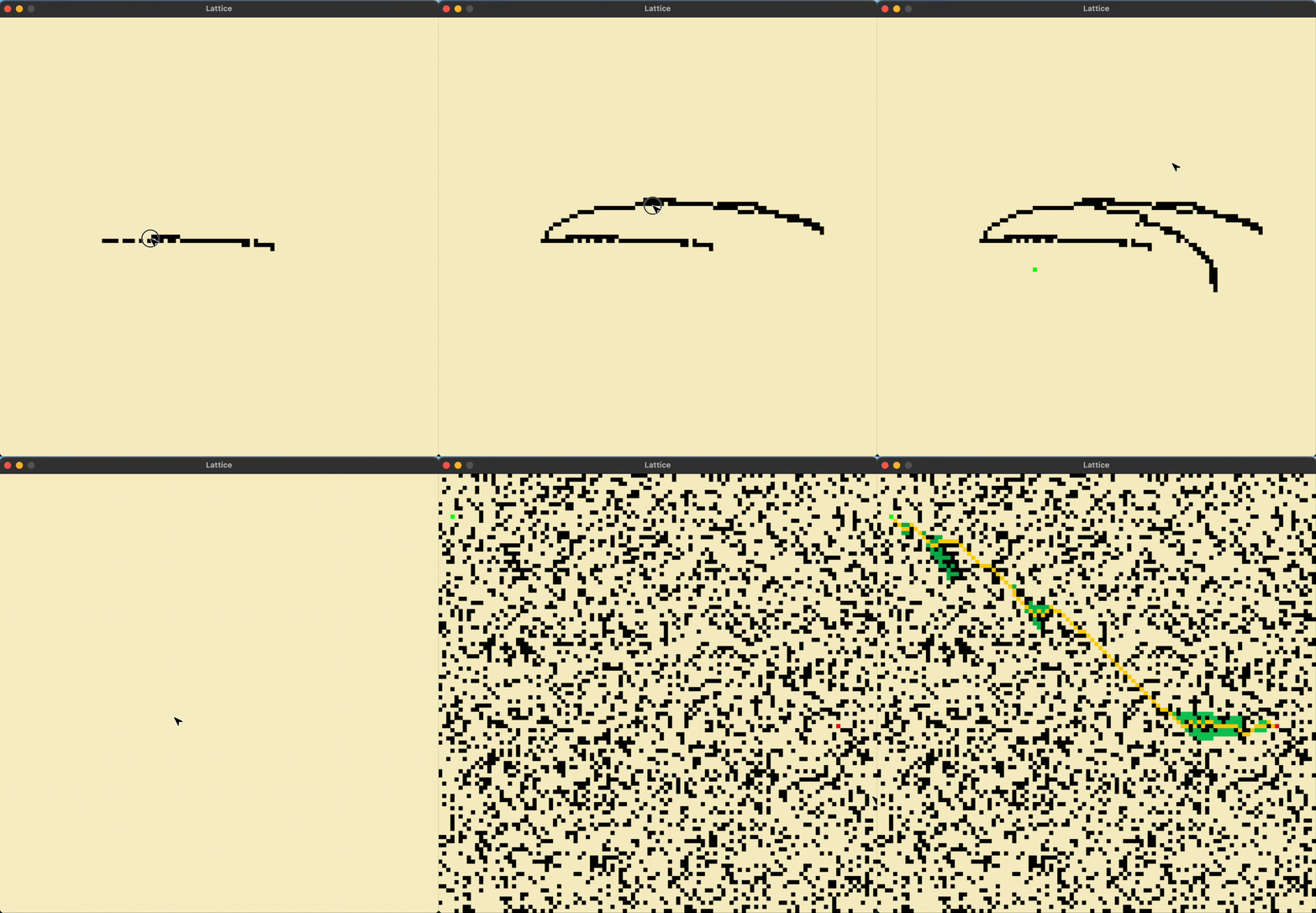
This is the most basic and common task that would be performed when using this application. Thus, whenever a mouse is pressed, we get the x and y coordinates from the screen, translate them to the particular row and column number (using the NODE_SIZE static value as reference), and changes that particular node's state to NodeState.WALL. When this is done, pygame.display.update() is also called, and all of this together renders walls on the screen. Since I wanted the user to be able to drag and create walls, I had to make use of a boolean variable, mouse_pressed. Whenever the mouse is pressed down, this value is set to true, and vice versa. Since pygame runs in a loop, while the mouse is held down, whereever the mouse is, a node's state is changed, and subsequently, that part of the screen is updated.
Since there can be different draw modes, i.e. drawing walls, drawing origin/goal nodes, or even erasing, I had to add in extra conditions, which change the current draw mode when certain keys are pressed. For example, if the mouse is dragged while pressing e on your keyboard, node states are set to VACANT. This effectively acts as an eraser. When o is held down, the origin node is drawn, and vice versa for the goal node, where you need to press down g.
# main.py
mouse_pressed = False
while True:
    for event in pg.event.get():
        if event.type == pg.MOUSEBUTTONDOWN and event.button == 1:
            mouse_pressed = True
        if event.type == pg.MOUSEBUTTONUP and event.button == 1:
            mouse_pressed = False
        if event.type == pg.KEYDOWN:
            lattice.set_draw_mode(
                event_key_to_draw_mode_mapping.get(
                    event.key, DrawMode.SET_WALL
                )
            )
        if mouse_pressed:
            x, y = pg.mouse.get_pos()
            r = x // lattice_info.node_size
            c = y // lattice_info.node_size
            pos = Pos(r, c)
            lattice.change_node_state_on_user_input(pos)

# enums.py
class DrawMode(Enum):
    SET_WALL = 0
    SET_ORIGIN = 1
    SET_VACANT = 2
    SET_GOAL = 3

# Lattice.py
draw_mode_to_node_state_mapping = {
    DrawMode.SET_WALL: NodeState.WALL,
    DrawMode.SET_ORIGIN: NodeState.ORIGIN,
    DrawMode.SET_VACANT: NodeState.VACANT,
    DrawMode.SET_GOAL: NodeState.GOAL,
}

class Lattice
    def __init__(self, ...):
        .
        .
        .

    def change_node_state_on_user_input(self, pos: Pos) -> None:
        node = self.values[pos.r][pos.c]
        new_state = draw_mode_to_node_state_mapping[
            self.draw_mode
        ]  # Get the appropriate NodeState based on draw_mode.

        # Conditions below restrict only one origin node and one goal node to be set.
        if new_state == NodeState.ORIGIN:
            if self.origin:
                self.update_node_state_and_render(self.origin, NodeState.VACANT)
            self.origin = node
        elif new_state == NodeState.GOAL:
            if self.goal:
                self.update_node_state_and_render(self.goal, NodeState.VACANT)
            self.goal = node
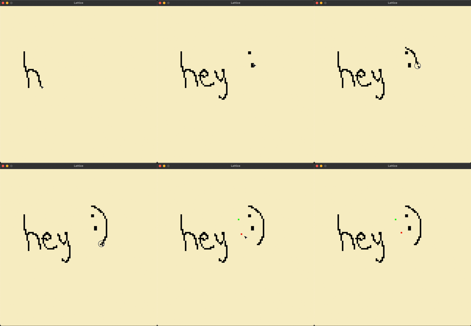
With all of this, we have a basic working grid on which we can draw stuff:
Pathfinding
Now it's time to get to the good stuff. Pathfinding algorithms. After all, they're the crux of this project. Let's start out with (arguably) the simplest, DFS.
Depth First Search
From Wikipedia:
The algorithm starts at the root node (selecting some arbitrary node as the root node in the case of a graph) and explores as far as possible along each branch before backtracking. Extra memory, usually a stack, is needed to keep track of the nodes discovered so far along a specified branch which helps in backtracking of the graph.
Let's do a quick revision on DFS. Here's the pseudocode, for an iterative implementation, and modified for the current usecase:
- Initialise a stack,
stack. - Push the root node onto the stack. In our case, this is the
originnode. - While the stack is not empty, do:
i) Pop
nodefrom stack. ii) Ifnodeequalsgoal, we've found a path fromorigintogoal. Returntrue. ii) Ifnodeis not visited and is not a wall node: a) Push both non-wall and unvisited neighbours ofnode,neighbour, into stack. b) Setneighbour's predecessor asnode, to enable backtracking after finding a path. - If stack is empty, return
False, since a path was not found.
How is the neighbour chosen for a particular node? We just look at the 8 neighbours surrounding a node, keeping in mind extra conditions for nodes that exist at the border. Here's the logic for choosing neighbour nodes:
def get_neighbours(self, node: Node) -> List[Node]:
    neighbours = []
    r, c = node.get_pos().r, node.get_pos().c
    if r > 0:
        neighbours.append(self.values[r - 1][c])
    if r < self.nrows - 1:
        neighbours.append(self.values[r + 1][c])
    if c > 0:
        neighbours.append(self.values[r][c - 1])
    if c < self.ncols - 1:
        neighbours.append(self.values[r][c + 1])
    return neighbours
Pretty self explanatory. Some people choose to go with implementations that don't take into account diagonal neighbours. But that's just an arbitrary decision. I chose to go with only taking into account the 4 closest neighbours and not any diagonal neighbours, because frankly, a path going through wall corners seems kinda weird. And your A* search becomes very boring to look at.
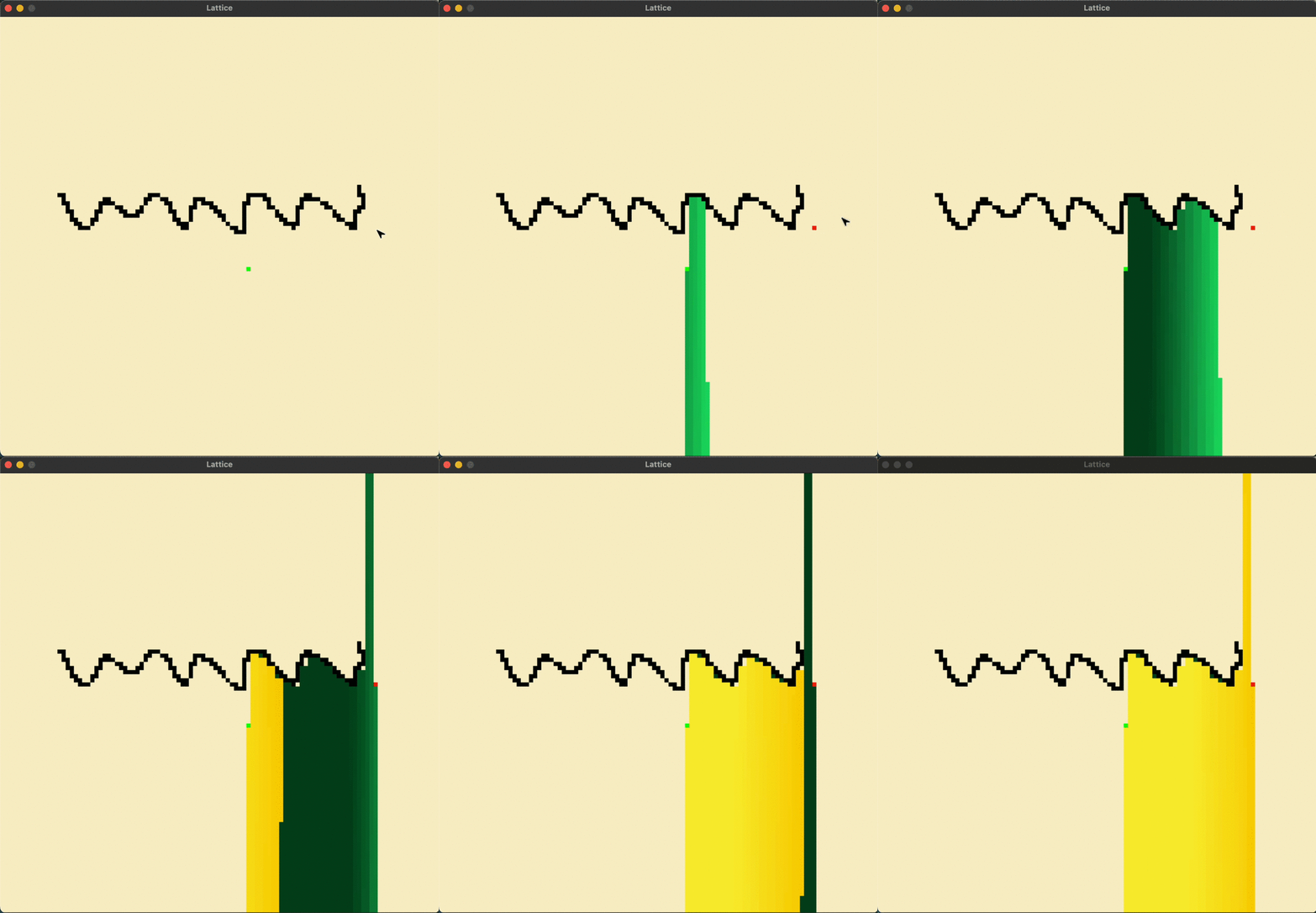
One important thing here is that since DFS uses a stack, it processes nodes in a first-come first-served basis. This means, the first if-condition in our function above biases the DFS algorithm in the direction it chooses to go. Since DFS does not have a heuristic of any sort, it does not make sense to choose which direction we want the algorithm to be biased in. Unlike A*, the algorithm has no clue where the goal node is, so it does not matter which direction it chooses to go in.
With that being said, here's the DFS algorithm in action:
On a grid with randomized walls:
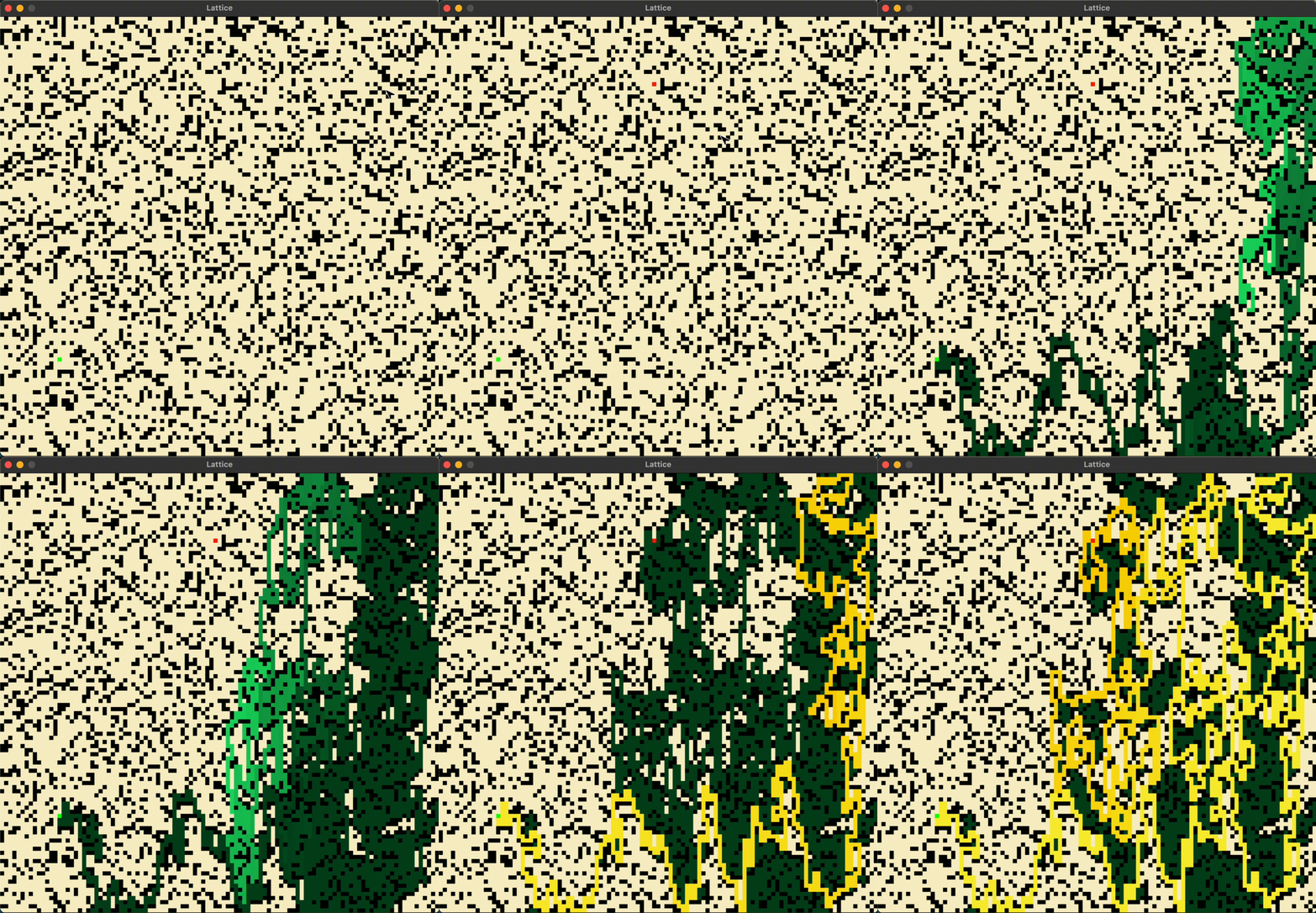
Doesn't look very efficient, huh? It shouldn't be. DFS just picks a direction and... goes at it. With no real thought about where it's heading. DFS works good for solving mazes, but for something like a 2D grid, it can lead to some unwieldly looking paths such as the one above. DFS has the possibility to get lost in an infinite branch and never make it to the solution node. Assuming we have infinite time, and it does traverse the entire graph, the final path might be infinitely long, even if the goal node was just beside the origin node. It does not guarantee the shortest path. You want the guaranteed shortest path, you say? Well, say hi to BFS.
Breadth First Search
Breadth-first search is an algorithm for searching a tree data structure for a node that satisfies a given property. It starts at the tree root and explores all nodes at the present depth prior to moving on to the nodes at the next depth level. Extra memory, usually a queue, is needed to keep track of the child nodes that were encountered but not yet explored.
The pseudocode for BFS is as follows:
- Initialise a
queue, enqueue the origin node. - For current nodes in
queue: i) Popnodeii) Ifnodeequalsgoal, path has been found. Returntrue. iii) Ifnodeis not visited and is not a wall a) Mark as visited b) For each neighbours ofnodewhich is not visited and is not a wall i) Pushneighbourontoqueueii) Setneighbour's predecessor asnode, to enable backtracking after finding a path. - If queue is empty, path has not been found, return
false
Unlike DFS where it picks a path and keeps doing along it until it no longer can, BFS visits it's neighbours, and the neighbours of it's neighbours, and so on until a path is found. There is still no heuristic, so it does not have any idea about where the goal node is, but alteast for this use-case, i.e. a 2D grid, on a randomized grid that is not maze-like, BFS performs better.
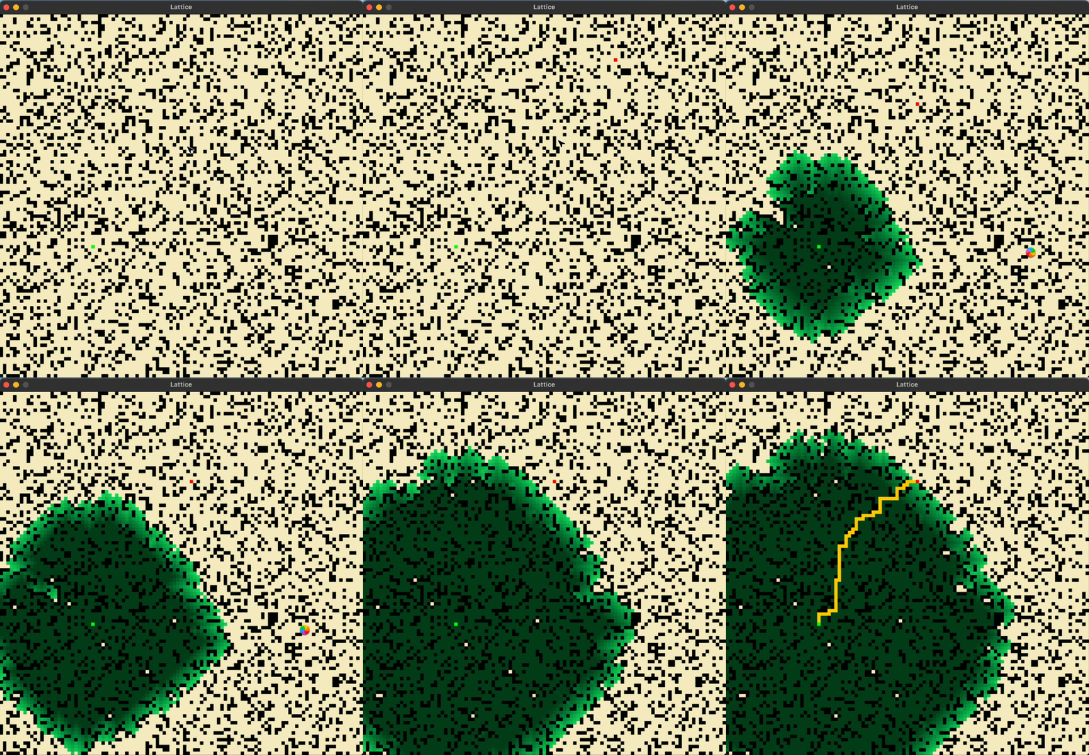
I promise the actual application isn't as laggy as what this GIF represents. When converting a .MOV to a .GIF, a lot of the frames are cut. I urge you to try the app out by cloning the repository and running the app locally.
Dijkstra's Shortest Path Algorithm
Dijkstra's algorithm is an algorithm for finding the shortest paths between nodes in a graph, which may represent, for example, road networks. It was conceived by computer scientist Edsger W. Dijkstra in 1956. The algorithm exists in many variants. Dijkstra's original algorithm found the shortest path between two given nodes, but a more common variant fixes a single node as the "source" node and finds shortest paths from the source to all other nodes in the graph, producing a shortest-path tree.
In my implementation, once a goal node is found, the algorithm terminates. We have no use in finding the distance to other nodes on the lattice.
And yes, before you say anything, yes, Dijkstra's algorithm is supposed to be used on weighted graphs. The lattice project consists of a grid of nodes- weights cannot be used here. While they can be randomnly assigned, it doesn't make any sense to, because 1) we cannot visualize them, and 2) all nodes exist equidistant from each other. Dijkstra's algorithm is supposed to be used on weighted graphs. The most common difference between Dijkstra's and BFS is the following: While BFS might choose any one of it's unvisited neighbours, Dijktra's chooses the one with the current lowest edge weight.
Since our implementation of Dijkstra's is on an unweighted graph, I assigned weights of 1 to every single node on the lattice. This means that effectively, Dijkstra's is the same as BFS. So I'll do you a favour and skip this section, because the next one is much more exciting.
A* Search
In comes the mighty heuristic.
A* (pronounced "A-star") is a graph traversal and path search algorithm, which is used in many fields of computer science due to its completeness, optimality, and optimal efficiency. One major practical drawback is its space complexity, as it stores all generated nodes in memory. Thus, in practical travel-routing systems, it is generally outperformed by algorithms which can pre-process the graph to attain better performance, as well as memory-bounded approaches; however, A* is still the best solution in many cases.
Our unweighted graph can actually be used as an example as to why Dijkstra's is bad on certain graphs. I highly recommend you watch Computerphile's video on A Star search. . In short, Dijkstra's algorithm is greedy. It only looks at the local current shortest path. Even if that path leads away from the goal, if the weights are small, Dijkstra will head in that direction. If we have a grid of interconnected nodes with very small and similar weights, Dijktra's will spend a lot of time in this area due to it's greedy nature. It is why in our usecase, it performs equally to BFS, which is not what we want.
Heuristic: Euclidean Distance
A heuristic here is some sort of information that tells the algorithm which direction the goal node is. A very simple heuristic to use here is the Euclidean distance to the goal node. Before the algorithm starts, we loop through all the nodes, and for each node, we calculate the heuristic by calculating the Euclidean distance between the current node and the goal node:
goal_pos = self.get_goal().get_pos()
x1, y1 = goal_pos.r, -goal_pos.c
for r in range(self.nrows):
    for c in range(self.ncols):
        node_pos = self.get_node(r, c).get_pos()
        x2, y2 = node_pos.r, -node_pos.c
        euclid_distance = math.sqrt(((x2 - x1) ** 2) + ((y2 - y1) ** 2))
        self.get_node(r, c).set_heuristic(euclid_distance)
Once we have this, we can begin the algorithm.
- Initialise a priority queue
dist, which keeps track of nodes and their distance from origin. - Add
originnode todist, set distance tooriginas 0. Setnodetoorigin. - While True:
i) Look at all unvisited neighbours of
node. ii) For eachneighbour: a) If the neighbour is thegoalnode, a path has been found, returnTrue. b) If the current distance to neighbour is lesser than it's previous distance (initially, this is infinite), update the new path distance usingdist[neighbour] = intiii) Choose the nextnode: a) Look at the priority queuedist. b) Choose the one at the top, i.e. out of all the visited nodes, choose the one with the smallest value of distance to node + heuristic value of node iv) If there are no nodes to visit, returnFalse, as path cannot be found.
This is by far the coolest algorithm to see visually, here's what it looks like in action:
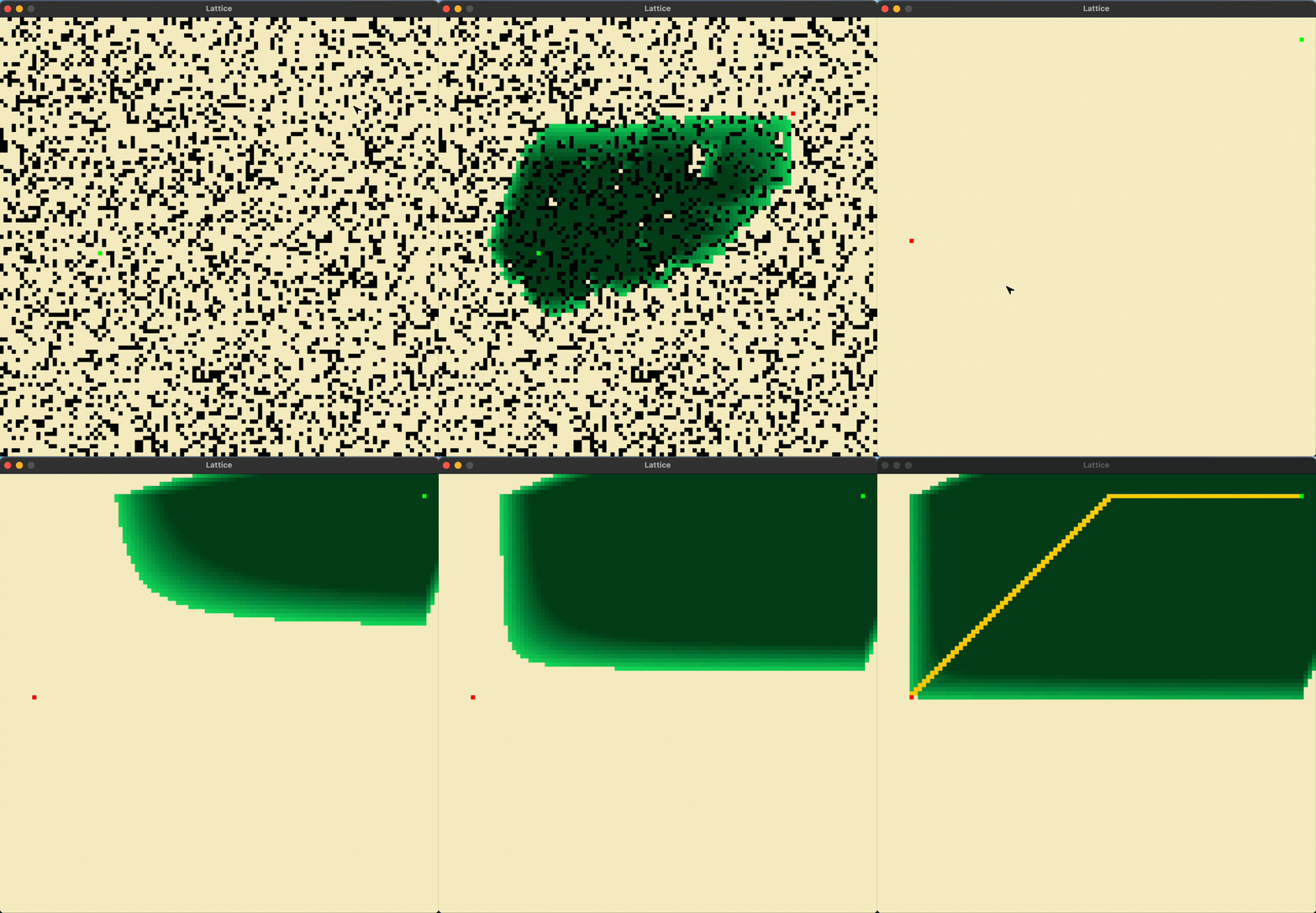
Look at that! It knows where to go. If you're thinking, which is still spreads out even though it knows where to go, it's because we only choose to look at the 4 neighbours that are touching any node. If we look at the all 8 Moore's neighbours of a node, A* goes through the grid like butter. But, it isn't very fun to look at. And the visualization makes it looks like it can go through walls. Which I don't fancy.
Maze Generation
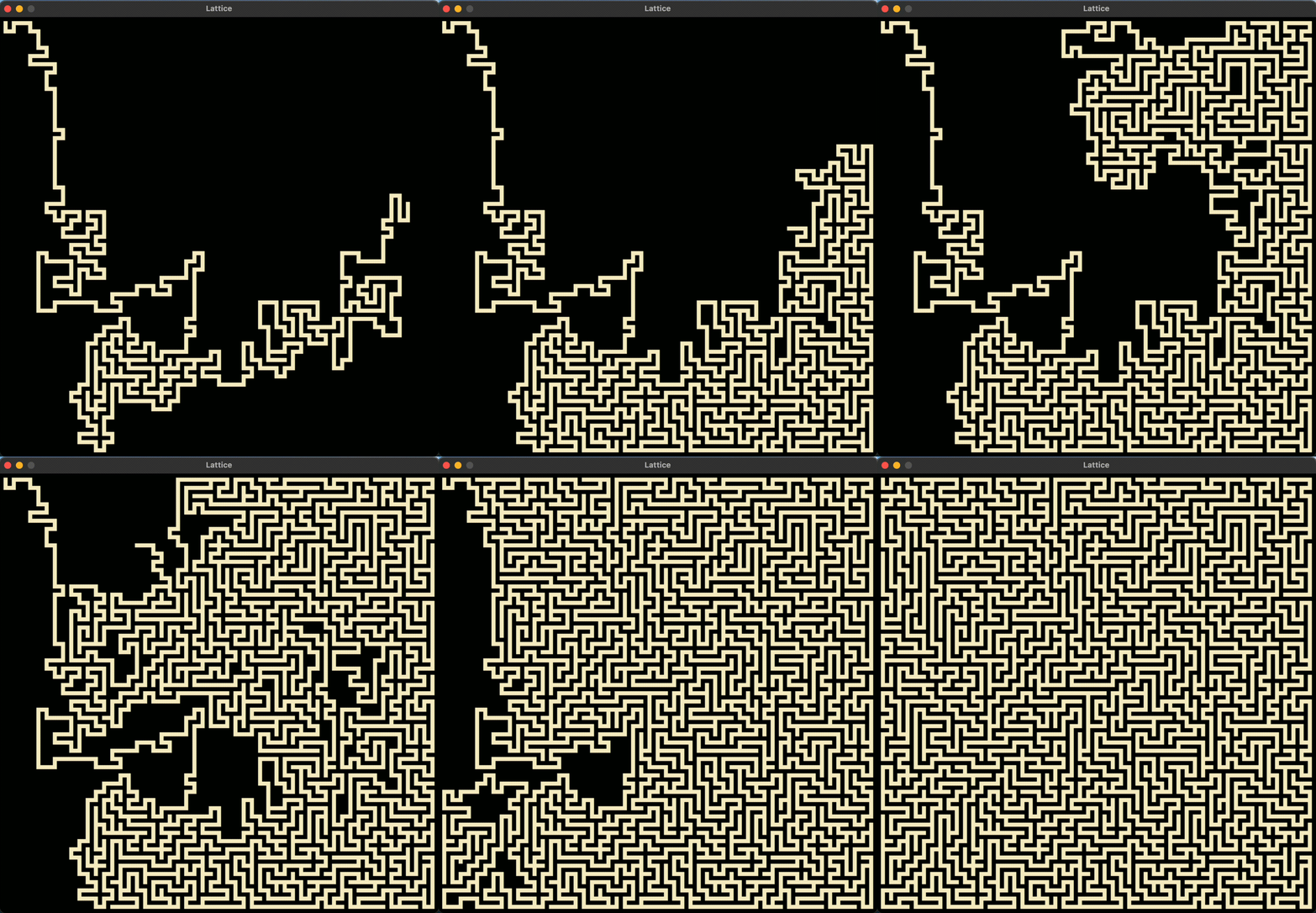
What's a pathfinding algorithm without a maze to test it out on? I read through the Wikipedia article on this topic and decided to implement the iterative version of the randomized depth-first search algorithm. What this is basically, is we start out on a completely filled grid, and we do a depth-first search. But instead of going down the first neighbour out of all the possible neighbours of a node, we randomly choose one and go down that route instead.
Since I was working with purely pseudocode, this part took me the longest to implement in code, simply because no other source out there mentioned how to do DFS with leaving walls in between nodes. Eventually I figured it out. I had to write a custom neighbour finding function which only considered neighbours one node away. When a neighboru was shortlisted, the algorithm would set that node to vacant, and also the node between this neighbour and the node we're currently at. This way, it carves out a path. Here's the custom neighbour finding algorithm:
def get_one_off_neighbours(self, node: Node) -> List:
    neighbours = []
    r, c = node.get_pos().r, node.get_pos().c
    if r > 1:
        neighbours.append(self.get_node(r - 2, c))
    if r < self.nrows - 2:
        neighbours.append(self.get_node(r + 2, c))
    if c > 1:
        neighbours.append(self.get_node(r, c - 2))
    if c < self.ncols - 2:
        neighbours.append(self.get_node(r, c + 2))
    return neighbours
And here's the maze generation in action, which if I so myself, looks hecking cool. One pre-computation that I did to improve efficiency is to calculate all neighbour indices for each index in the lattice. This way, we don't have to calculate the neighour index for each node during each state of the Game of Life.
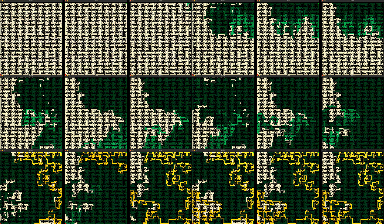
And here's each of the 3 algorithms: DFS, BFS, and A star, visualized on the maze. The origin node is at the top right while the goal node is on the bottom left.
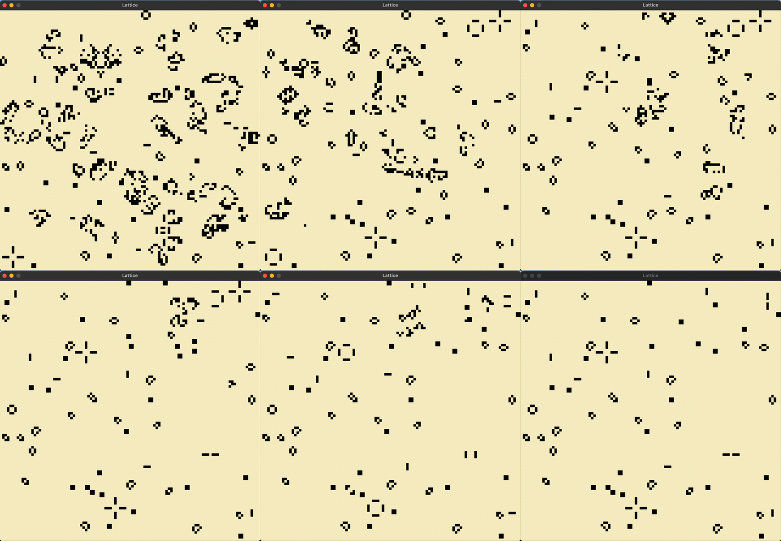
Game of Life
While I was at it, I thought, hey, why not visualize Conway's Game of Life. And so I did.
The Game of Life, also known simply as Life, is a cellular automaton devised by the British mathematician John Horton Conway in 1970. It is a zero-player game, meaning that its evolution is determined by its initial state, requiring no further input. One interacts with the Game of Life by creating an initial configuration and observing how it evolves. It is Turing complete and can simulate a universal constructor or any other Turing machine.
The Game of Life is one of the coolest things I've ever seen and it leaves me in awe to see how something with such simple rules can be used to simulate life itself. And since the game is Turing complete , you can theoetically build any software system in the world today using the Game of Life. I urge you to watch these following videos that depict how mindblowing this thing truly is:
The algorithm is pretty concise and easy to implement, here's all the code you need to emulate it:
def game_of_life(self) -> None:
    # Pre-calculating neighbour indices, so that it isn't done every generation. Sure, uses a lot more storage but that isn't a bottleneck.
    positions = [
        [0, 1],
        [0, -1],
        [1, -1],
        [-1, 1],
        [1, 1],
        [-1, -1],
        [1, 0],
        [-1, 0],
    ]
    all_neighbour_indices = {}
    for r in range(self.nrows):
        for c in range(self.ncols):
            neighbour_indices = []
            for position in positions:
                new_r = r + position[0]
                new_c = c + position[1]
                if (
                    new_r >= 0
                    and new_r < self.nrows
                    and new_c >= 0
                    and new_c < self.ncols
                ):
                    neighbour_indices.append([new_r, new_c])
            all_neighbour_indices[self.values[r][c]] = neighbour_indices

    prev_nodes_to_update = []  # Checks if evolution has stopped.
    evolution_stopped = False
    while not evolution_stopped:
        batch_update_list = (
            []
        )  # Since each generation is a pure function of the preceding one, we have to update the node states only after going through all of them once.
        # A node's next-generation state shouldn't influence any current-generation node's state.
        for r in range(self.nrows):
            for c in range(self.ncols):
                node = self.get_node(r, c)
                neighbour_indices = all_neighbour_indices[node]
                num_live_neighbours = self.get_num_live_neighbours(
                    neighbour_indices
                )
                is_node_alive = node.get_state() == NodeState.WALL
                if is_node_alive:
                    if num_live_neighbours < 2 or num_live_neighbours > 3:
                        batch_update_list.append([node, NodeState.VACANT])
                elif not is_node_alive and num_live_neighbours == 3:
                    batch_update_list.append([node, NodeState.WALL])
        nodes_to_update = []
        for item in batch_update_list:
            node, new_state = item
            node.set_state(new_state)
            nodes_to_update.append(node)

        # Takes care of termination state. I wrote this in a jiffy and I don't know how it works and I'm too lazy to try understanding. But hey, it works (almost all the time) So I'm not touching it.
        for item in prev_nodes_to_update:
            if nodes_to_update == item:
                evolution_stopped = True
        if len(prev_nodes_to_update) == 2:
            prev_nodes_to_update.pop(0)
        prev_nodes_to_update.append(nodes_to_update)

        self.render_nodes(nodes_to_update)
Future Work
That's all. For now. In the future, I plan to expand on more pathfinding and maze generation algorithms, specifically, Iteratively Deepening DFS, and Prim's/Kruskal's for maze generation. Try the program out yourself, and let me know what you think!